Crossflow Fin and Tube Heat Exchanger - Finite Volume Model

Model description

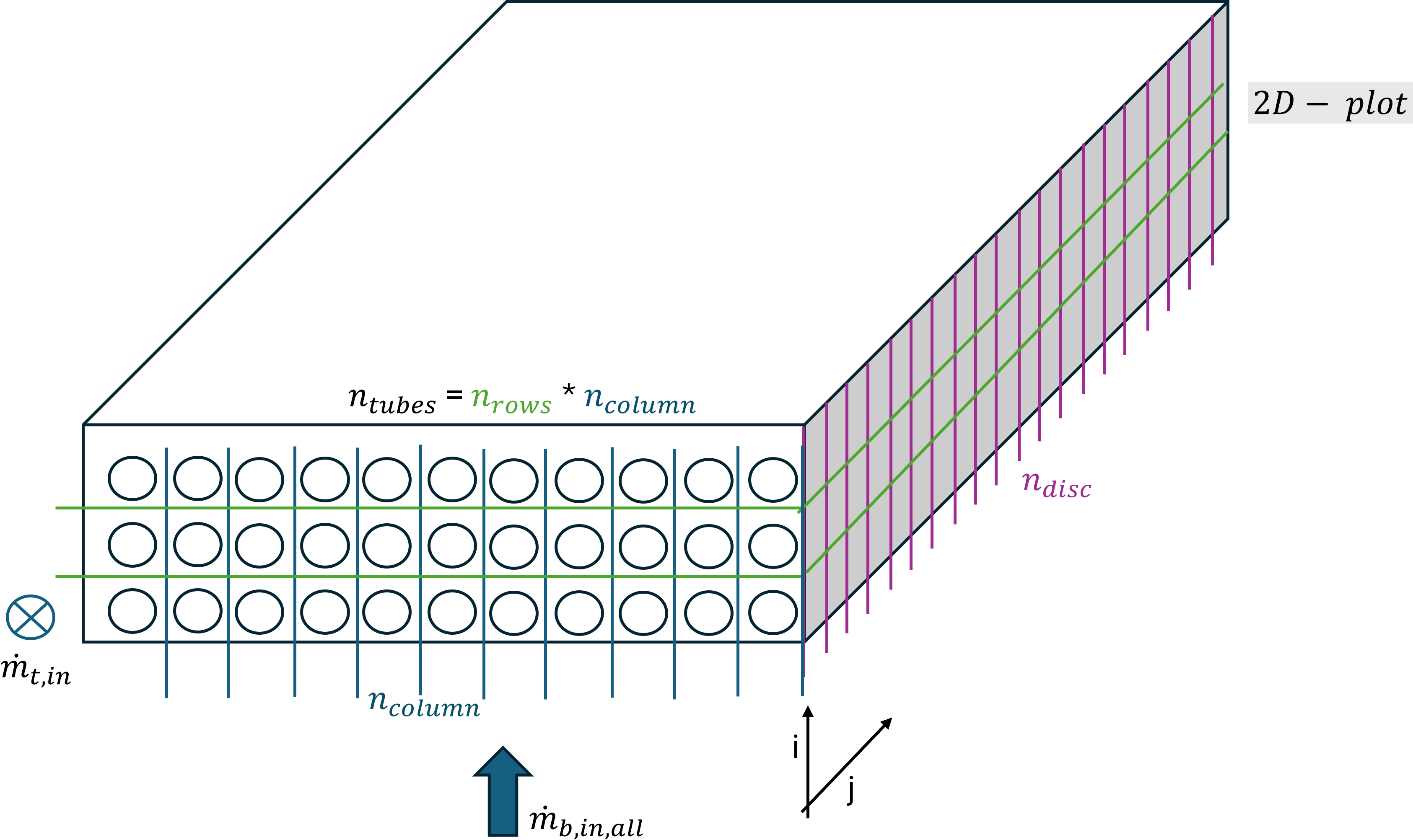
The model geometrical implementation is similar to the model with 8 circuits from the reference [1] (see Figure 17).

Class description

class component.heat_exchanger.hex_crossflowfintube_finitevolume.HexCrossFlowTubeAndFinsFiniteVolume

Component: Cross-Flow Tube-and-Fins Heat Exchanger (Hex)

Model: Discretized Cross-Flow Heat Exchanger with Fin Efficiency and Pressure Drop

Description:

This model simulates a cross-flow heat exchanger with tube-and-fins geometry, suitable for systems where one fluid flows through tubes and the other over an external finned surface. The model uses detailed correlations for heat transfer coefficients and pressure drops, accounting for phase change phenomena (condensation and evaporation). It is designed for steady-state, on-design simulations. The model uses a finite volume discretization to take into consideration the fluid properties evolution accross the heat exchanger.

Assumptions:

• Steady-state operation.

• Uniform flow distribution across tubes and fins.

• Correlations used for heat transfer and pressure drop calculations (e.g., Gnielinski, Müller-Steinhagen-Heck).

• Two-phase flow effects are considered where applicable.

• Fluid properties are retrieved from CoolProp.

Connectors:

su_H (MassConnector): Mass connector for the hot-side supply (tube or fin side depending on configuration). su_C (MassConnector): Mass connector for the cold-side supply (tube or fin side depending on configuration).

ex_H (MassConnector): Mass connector for the hot-side exhaust. ex_C (MassConnector): Mass connector for the cold-side exhaust.

Q (HeatConnector): Heat connection (not actively used in current implementation).

Parameters:

H_DP_ON (bool): Flag to enable pressure drop calculation on hot side. C_DP_ON (bool): Flag to enable pressure drop calculation on cold side. n_disc (int): Number of discretization segments along the heat exchanger length. Fin_Side (str): Specifies which side has fins (‘H’ for hot side, ‘C’ for cold side).

Geometry Parameters:

Fin_OD : Fin diameter/length [m]

Fin_per_m : Fin density per m [1/m]

Fin_t : Fin Thickness : [m]

Fin_type : ‘Annular’ or ‘Square’

fouling : Global fouling resistance [K/W]

h : Bundle height [m]

k_fin : Fin thermal conductivity [W/(m*K)]

pitch_V : Vertical Pitch [m]

pitch_H : Horizontal Pitch [m]

tube_arrang : Tube arrangement ‘Inline’ or ‘Staggered’

Tube_cond : Tube material conductivity [W/(m*K)]

Tube_L : Tube length [m]

Tube_OD : Tube outer diameter [m]

Tube_t : Tube thickness [m]

w : Bundle width [m]

Fin_Side : Fin side ‘H’ or ‘C’

Inputs:

fluid_H (str): Hot-side fluid.

h_su_H (float): Hot-side inlet specific enthalpy [J/kg].

P_su_H (float): Hot-side inlet pressure [Pa].

m_dot_H (float): Hot-side mass flow rate [kg/s].

fluid_C (str): Cold-side fluid.

h_su_C (float): Cold-side inlet specific enthalpy [J/kg].

P_su_C (float): Cold-side inlet pressure [Pa].

m_dot_C (float): Cold-side mass flow rate [kg/s].

Outputs:

h_ex_C: Cold exhaust side enthalpy. [J/kg]

P_ex_C: Cold exhaust side pressure. [Pa]

h_ex_H: Hot exhaust side enthalpy. [J/kg]

P_ex_H: Hot exhaust side pressure. [Pa]

Q_dot: Heat Exchanger’s heat duty. [W]

M_tube: Total mass inventory in the tube-side [kg].

M_bank: Total mass inventory in the fin-side (bundle side) [kg].

T_matrix, H_matrix, P_matrix, x_matrix: Discretized distributions of temperature, enthalpy, pressure, and vapor quality within the heat exchanger.

Example of use

import matplotlib.pyplot as plt
from CoolProp.CoolProp import PropsSI
from labothappy.component.heat_exchanger.hex_crossflowfintube_finitevolume import HexCrossFlowTubeAndFinsFiniteVolume

pressure_plot = 1
temperature_plot = 1

"--------- 1) Data ------------------------------------------------------------------------------------------"

"Cyclopentane Su"
ACC = HexCrossFlowTubeAndFinsFiniteVolume()

T_in_air = 15 + 273.15
P_in_air = 101325

rho_in_air = PropsSI('D', 'T',T_in_air, 'P', P_in_air, 'Air')

V_dot = 8 # m^3/s
m_dot_air = V_dot*rho_in_air

# Evaporator Case
ACC.set_inputs(
  
    # First fluid
    fluid_H = "Cyclopentane",
    T_su_H = 65 + 273.15, # K
    P_su_H = 116645.96, # Pa
    # x_su_H = 0.5, # Quality 
    m_dot_H = 0.5, # kg/s

    # Second fluid
    fluid_C = "Air",
    T_su_C = T_in_air, # K
    P_su_C = P_in_air, # Pa
    m_dot_C = m_dot_air, # kg/s  # Make sure to include fluid information
)

"Geometry"

ACC.set_parameters(
    Fin_OD = 0.0218694, # m
    Fin_per_m = 315, # 1/m
    Fin_t = 0.00033, # m
    Fin_type = 'Square',
    fouling = 0, 
    h = 0.5, # m 
    k_fin = 230, # W/(m^2*K)
    pitch_V = 0.024765, # m 
    pitch_H = 0.024765, # m 
    tube_arrang = 'Staggered', 
    Tube_cond = 50, # W/(m^2*K) 
    Tube_L = 0.6, # m 
    Tube_OD = 0.0102, # m
    Tube_pass = 1,
    Tube_t = 0.001, # m
    w = 1, # m
 
    Fin_Side = 'C', H_DP_ON = True, C_DP_ON = True, n_disc = 100)
 
ACC.solve()

if temperature_plot == 1:
    # Plot the temperature matrix for the tube side
    plt.figure(figsize=(8, 6))  # Optional: set figure size
    plt.pcolor(ACC.T_matrix, shading='auto', cmap='jet')  # Better colormap and shading
    plt.title('Temperature Distribution')
    plt.xlabel('Disc Index')
    plt.ylabel('Row Index')
    plt.colorbar(label='Temperature [°C]')  # or K, depending on your units
    plt.tight_layout()
    plt.show()

if pressure_plot == 1:
    #Plot the pressure drop evolution
    import matplotlib.pyplot as plt
    import numpy as np
    
    # Slice the matrix
    tube_side_mask = np.zeros_like(ACC.P_matrix, dtype=bool)
    bank_side_mask = np.zeros_like(ACC.P_matrix, dtype=bool)
    
    tube_side_mask[1::2, :] = True
    bank_side_mask[0::2, :] = True
    
    tube_side_values = np.ma.masked_where(~tube_side_mask, ACC.P_matrix)
    bank_side_values = np.ma.masked_where(~bank_side_mask, ACC.P_matrix)
    
    # Create figure
    fig, ax = plt.subplots(figsize=(10, 6))
    
    # Plot both matrices
    tube_cmap = ax.imshow(tube_side_values, cmap='viridis', aspect='auto', origin='lower')
    bank_cmap = ax.imshow(bank_side_values, cmap='plasma', aspect='auto', origin='lower')
    
    # Add colorbars
    cbar_tube = plt.colorbar(tube_cmap, ax=ax, orientation='vertical', pad=0.02)
    cbar_tube.set_label('Tube Side Pressure [Pa]')
    
    cbar_bank = plt.colorbar(bank_cmap, ax=ax, orientation='vertical', pad=0.12)
    cbar_bank.set_label('Bank Side Pressure [Pa]')
    
    # Labels
    ax.set_title('Pressure Distribution: Tube Side vs Bank Side')
    ax.set_xlabel('Disc Index')
    ax.set_ylabel('Row Index')
    
    plt.tight_layout()
    plt.show()
    
    ACC.print_setup()
    print("=== Heat Exchanger outlet conditions ===")
    print(f"ex bundle: fluid_bundle = {ACC.B_su.fluid}, T_ex_bundle ={(int(round(ACC.B_ex.T)))}[K], h_ex_bundle={(int(round(ACC.B_ex.h)))}[J/kg-K], p_ex_bundle={(int(round(ACC.B_ex.p)))}[Pa], m_dot_ex_bundle={(int(round(ACC.B_su.m_dot)))}[kg/s]")
    print("======")
    print(f"ex tube: fluid={ACC.T_su.fluid}, T_ex_tube ={(int(round(ACC.T_ex.T)))}[K], h_ex_tube={(int(round(ACC.T_ex.h)))}[J/kg-K], p_ex_tube={(int(round(ACC.T_ex.p)))}[Pa], m_dot_tube={ACC.T_su.m_dot}[kg/s]")

References

[1] S. Macchitella, G. Colangelo, and G. Starace, ‘Performance Prediction of Plate-Finned Tube Heat Exchangers for Refrigeration: A Review on Modeling and Optimization Methods’, Energies, vol. 16, no. 4, p. 1948, Feb. 2023, doi: 10.3390/en16041948.